
Research
Ephris: Stronger In-Context Learning on Graphs with Linear Scaling
On this page
A graph already tells us how its nodes are connected. Can a pretrained model use those connections to learn from labeled examples at scale?
Ephris is our answer. It uses sparse message passing to predict unknown node labels from a graph and its labeled examples, without updating its pretrained weights.
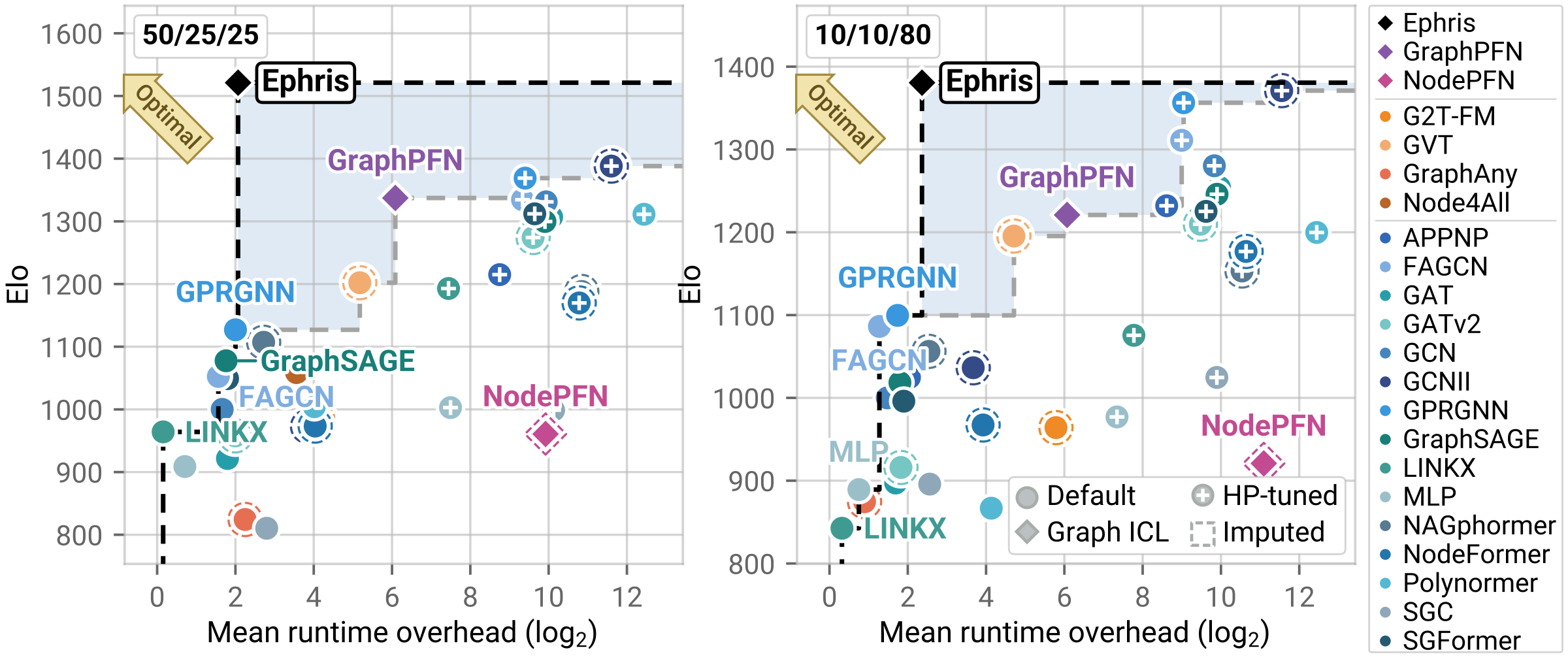
Across 51 node-classification datasets, Ephris ranks first overall among the models we evaluated. The plot above shows its performance alongside adaptation time. Its computation also scales linearly in feature entries and edges.
What is graph in-context learning?
A tabular foundation model uses labeled rows in a new table to predict labels for the remaining rows. Those labeled rows form the context: examples from which the model infers the task, without retraining.
Graph in-context learning extends this idea to connected data. Nodes play the role of rows, with features describing each node and edges connecting them. Known node labels provide the context.
For example, suppose we want to predict the topics of research papers. Given topic labels for some papers, the model predicts topics for the rest using:
- Node features: numerical descriptions of each paper.
- Edges: citations connecting the papers.
- Context labels: the known topics of some papers.
The model sees features and connections for every node. The labels it is asked to predict stay hidden.
NodePFN and GraphPFN build on tabular foundation models. NodePFN adds a message-passing branch to TabPFN, and GraphPFN adds graph-attention adapters to LimiX. Both incorporate graph structure while retaining dense attention over context nodes.
Does a graph need attention between every pair?
Dense attention lets a tabular model compare rows and learn relationships between them. But the number of pairwise comparisons grows quadratically with the context size. If the labeled fraction stays fixed, doubling the graph size means roughly four times as many context pairs.
A graph already provides connections through which nodes can share information. In our paper example, a citation connects papers that may have related topics.
We built Ephris around sparse message passing to use those connections for in-context learning. The model learns how to use information from graph neighborhoods, avoiding dense attention across all node pairs.
How Ephris uses the graph
In Ephris, each node combines its own features with information from its neighbors. Known labels provide the context for predicting unknown ones.
Graph structure also shapes how the model processes features:
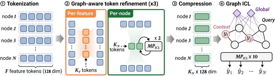
- Encode features and known labels. Each feature value becomes a learned token; known labels receive their own embeddings.
- Refine features using the dataset and graph. Summary tokens capture feature distributions. Node summaries exchange information over graph edges and feed it back into the feature tokens.
- Compress each node. The refined features are combined into a fixed-size representation, so the model can work with different numbers of features.
- Predict missing labels. Message-passing blocks combine features, connections, and labeled examples. A shared prediction head outputs class probabilities for the unlabeled nodes.
Graph structure guides both feature compression and label prediction.
A few model details
The evaluated model has 50.16 million parameters. It uses three feature-refinement blocks, compresses each node to 512 dimensions, and applies ten message-passing blocks. Each message-passing block includes eight global nodes.
The prediction head handles up to ten classes directly. For tasks with more classes, a fixed coding scheme divides the task into smaller classification problems and combines their probabilities, using the same pretrained weights.
Learning from synthetic graph tasks
We pretrained Ephris on 3.84 million synthetic graph tasks to teach it how to use labeled examples. No real benchmark datasets were used in pretraining.
The generator varies the graph structure and the relationships among features and labels. Graphs can contain communities, hubs, or paths. Tasks also vary how information spreads through the graph, from gradual propagation to cascades and effects that depend on how nodes are connected.
In each task, the model sees some labels and predicts the rest. Across millions of these tasks, it learns to infer a prediction rule from a new set of examples.
Stronger predictions across 51 datasets
We evaluated Ephris on 51 node-classification datasets across six application domains, comparing it with 15 graph neural networks (GNNs) and six graph foundation models. The tuned GNNs used an extensive hyperparameter search on validation data.
Elo summarizes pairwise model comparisons across datasets. Ephris has the highest Elo with both 50% and 10% labeled context.
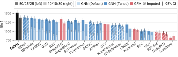
Ephris also ranks first on improvability, average rank, and average accuracy in both settings. Its lead over tuned GNNs narrows with less labeled context, but it remains ahead overall.
Performance and runtime
The next plot compares the time needed to apply each model to a new dataset with improvability, the normalized performance gap to the best model. Lower is better on both axes. Initial pretraining is excluded.
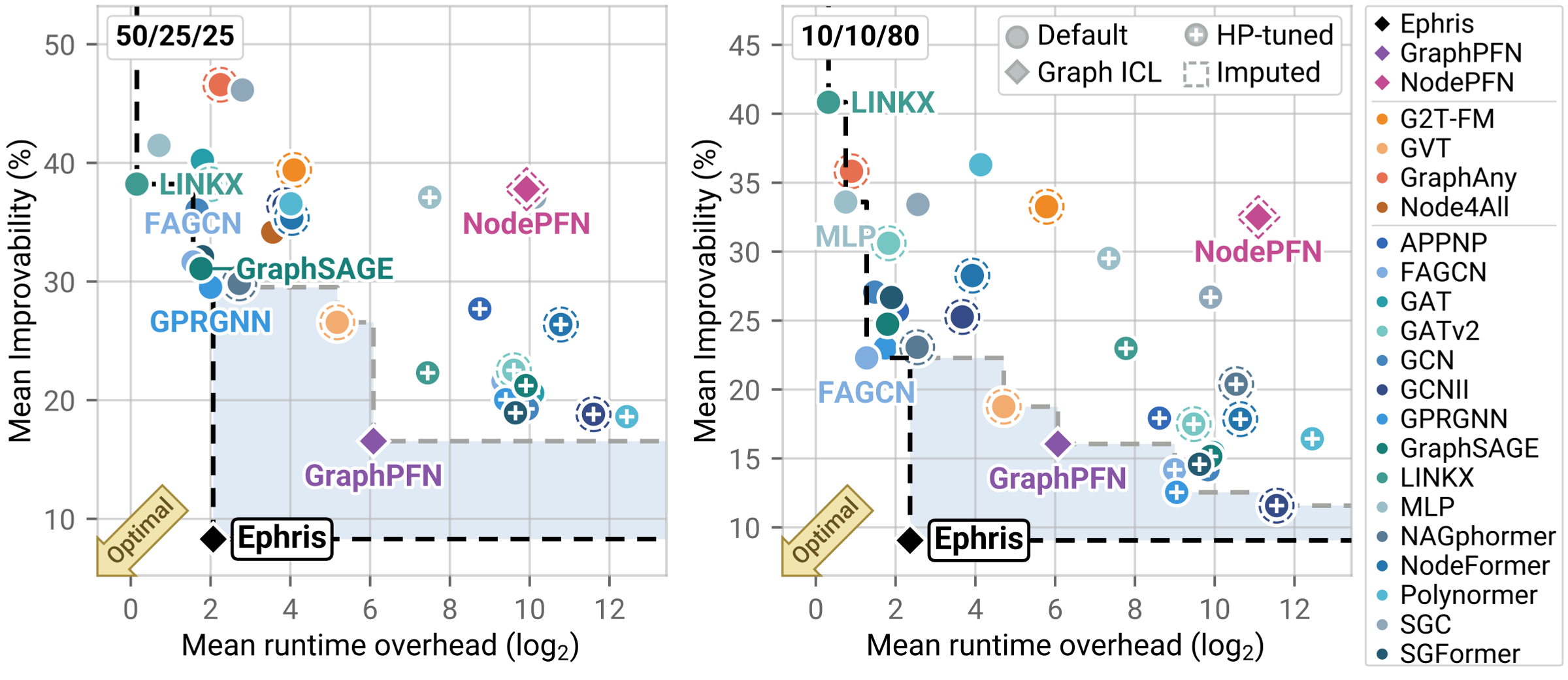
Ephris improves the trade-off in both label settings. Its adaptation time is much lower than GraphPFN's and in the same general range as training a single GNN once.
Evaluation details
We used train/validation/test proportions of 50/25/25 and 10/10/80, with five splits per setting. Ephris used training labels as context. Supervised baselines used validation labels for model selection and early stopping; each tuned GNN selected from 200 configurations.
Elo is a relative rating based on pairwise outcomes across datasets. Elo, improvability, and average rank use AUROC on binary tasks and accuracy on multiclass tasks. Average accuracy uses accuracy throughout. Elo intervals are 95% confidence intervals; hatched bars include imputed default GCN scores for runs that exhausted memory.
Runtime covers adaptation to each dataset: a single training run for default GNNs, the hyperparameter search for tuned GNNs, and each foundation model's adaptation procedure. It excludes initial pretraining.
Scalability
Ephris processes feature entries and passes messages along edges, with a fixed number of summary tokens and global nodes.
For a graph with N nodes, F features per node, and E edges, a prediction pass costs O(NF + E) when model dimensions, token counts, and depth are fixed. Here, NF counts feature entries and E counts edges. The cost is linear in the input size; a dense graph can still have quadratically many edges.
To measure scaling directly, we increased synthetic graph size from 50,000 to 500,000 nodes, keeping feature count, average degree, and labeled fraction fixed:
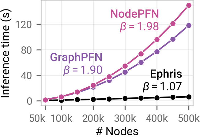
Ephris grows nearly linearly over the measured range, while NodePFN and GraphPFN grow nearly quadratically. The runtime gap widens as the graphs grow.
Scaling experiment details
Graphs had 32 features per node, average degree 8, and 50% labeled context. Each point is the median over three seeds on a single NVIDIA H200, without ensembling. Timing includes preprocessing and inference but excludes model loading. The fitted exponent describes growth over the measured range.
Performance across different graphs
To see how performance varies between datasets, we grouped them by graph size, feature count, class count, and how often connected nodes share a label.
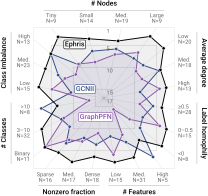
Ephris performs well across most groups. Tuned GCNII has the advantage in the groups with at least 5,000 features or more than ten classes, both outside the ranges seen during pretraining.
These gaps suggest where broader pretraining could help.
What comes next?
We want to build on these results in two directions.
Beyond node classification. How can we extend scalable graph in-context learning to edge-level and graph-level tasks? Predicting a connection or classifying an entire graph changes how we represent labeled examples and use them as context.
Discovering relationships in tables. In tabular data, we usually don't have an explicit graph. Can we discover useful, sparse connections between rows and use them for in-context learning? If we can build those connections efficiently, could they make tabular foundation models more scalable while preserving predictive performance?
Cite this work
Dooho Lee, Jinmo Lee, Minho Jeong, Kijung Shin, and Jaemin Yoo. (2026). Message Passing Does More with Less for In-Context Learning on Graphs. arXiv:2609.37057.
References
-
TabPFN. Noah Hollmann, Samuel Müller, Katharina Eggensperger, and Frank Hutter. (2023). TabPFN: A Transformer That Solves Small Tabular Classification Problems in a Second. ICLR.
-
NodePFN. Jeongwhan Choi, Jongwoo Kim, Woosung Kang, and Noseong Park. (2026). Learning Posterior Predictive Distributions for Node Classification from Synthetic Graph Priors. ICLR.
-
GraphPFN. Dmitry Eremeev, Oleg Platonov, Gleb Bazhenov, Artem Babenko, and Liudmila Prokhorenkova. (2026). GraphPFN: A Prior-Data Fitted Graph Foundation Model. ICML.
-
LimiX. Xingxuan Zhang et al. (2025). LimiX: Unleashing Structured-Data Modeling Capability for Generalist Intelligence. arXiv:2509.03505.
-
GCN. Thomas N. Kipf and Max Welling. (2017). Semi-Supervised Classification with Graph Convolutional Networks. ICLR.
-
GCNII. Ming Chen, Zhewei Wei, Zengfeng Huang, Bolin Ding, and Yaliang Li. (2020). Simple and Deep Graph Convolutional Networks. ICML.