Can a Tabular Foundation Model Complete an Image?

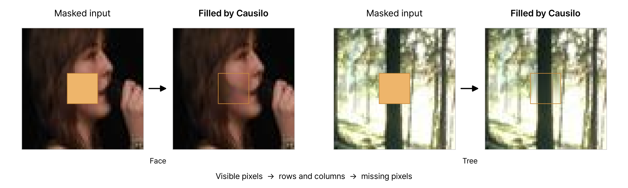
Close-ups of Causilo's predictions. Each panel shows a 64 × 64 region of a 256 × 256 photograph. The orange square marks the 16 × 16 missing region.

Causilo is a pretrained predictor for tables. Could we use it to fill in missing parts of an image?

It was pretrained entirely on synthetic tables and had never seen these photographs.

The photographs above show two of its reconstructions. The cheek has roughly the right color and shading, and the tree trunk continues through the gap. Both reconstructions are blurry, but some of the structure is there.

How did a tabular model fill those gaps? The first step was to decide how to represent an image as a table.

How does an image become a table?

In a grayscale image, each pixel has an x coordinate, a y coordinate, and a brightness value. We put each pixel in a row, with one column for each of these values.

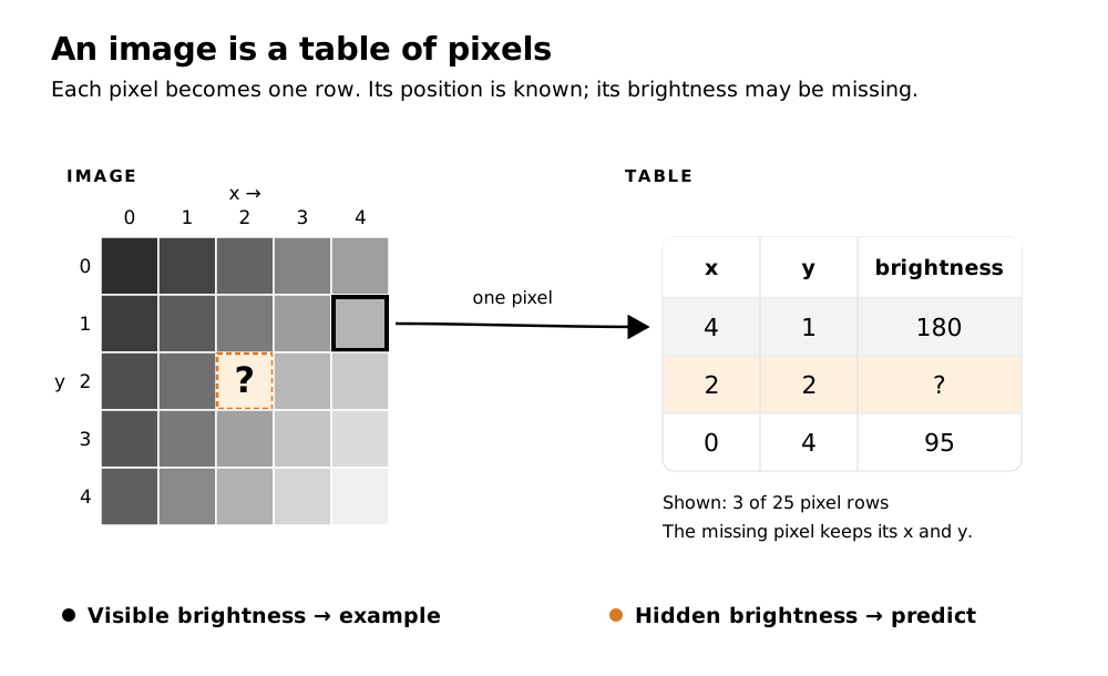
Visible pixels have values in all three columns. For hidden pixels, we know x and y but leave brightness blank. Causilo predicts those missing brightness values.

The visible rows form the model's context. Causilo uses these examples to make predictions without updating its pretrained weights.

We put each prediction back at its pixel's location to reconstruct the image.

We started with simple shapes to see what Causilo could infer from pixel positions alone.

Can it connect a line?

We drew horizontal, vertical, and diagonal lines, then hid a square in the middle of each image.

Each image is 64 × 64 pixels. A central 16 × 16 hole leaves 3,840 visible examples and 256 brightness values to predict. We first supplied only x and y, normalized from 0 to 1.

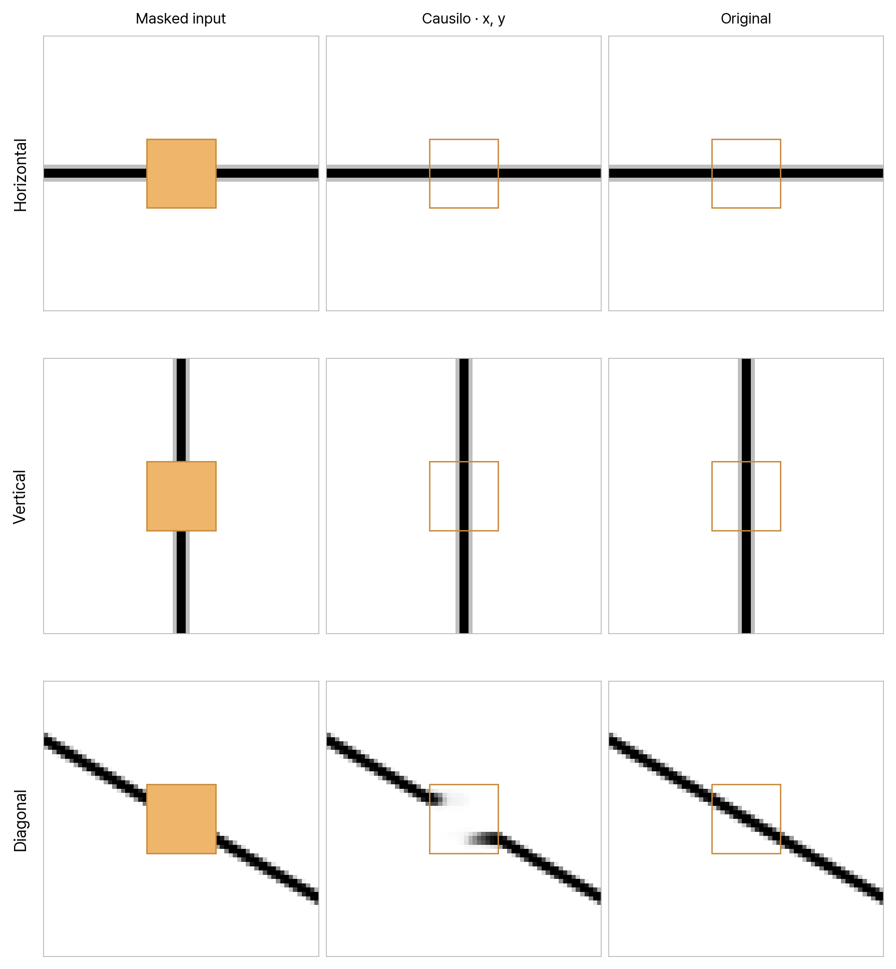
Causilo reconstructed the horizontal and vertical lines almost exactly. It struggled with the diagonal, even though the visible parts of the line continued on both sides of the hole.

For a horizontal line, brightness depends mainly on y. For a vertical line, it depends mainly on x. A diagonal requires a relationship between the two.

Rotated coordinates for the diagonal

We tried measuring each pixel's position along a tilted pair of axes.

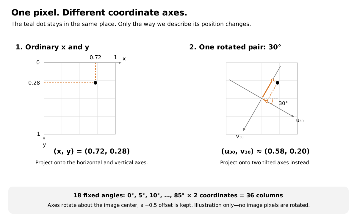
In the right coordinate system, a diagonal becomes as simple as a horizontal or vertical line: its brightness depends mainly on a single coordinate.

We used 18 coordinate pairs at 0°, 5°, …, 85°, giving 36 columns. The 0° pair is the original x and y. The image stays in place; we measure each position along several sets of axes.

These angles are fixed for every image. The diagonal in this example is at 30°, one of the included directions. All features are calculated from position alone, with the visible brightness values and row order held fixed.

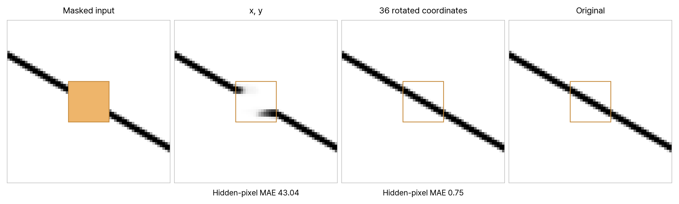
The diagonal now connects across the gap. Its mean absolute error (MAE) drops from 43.04 to 0.75.

MAE is the average absolute difference between predicted and original brightness inside the hole. Brightness ranges from 0 to 255, and lower MAE is better.

We used the same model and visible pixels. Only the positional features changed.

Can it complete a circle?

The rotated coordinates reconnected the diagonal. We next tried the same 36 features on a circle, again hiding a 16 × 16 square.

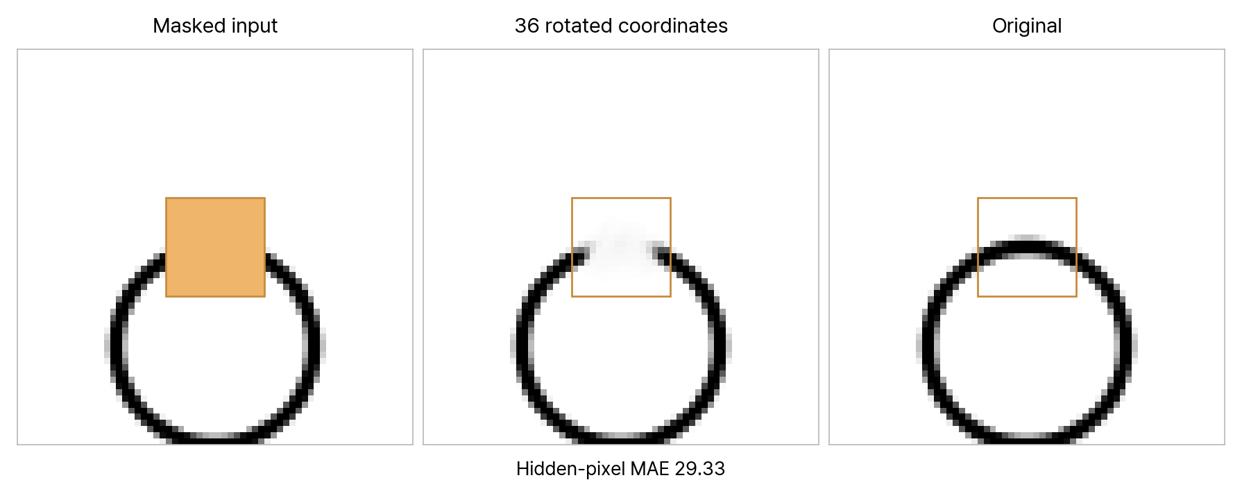
This time, the predicted stroke fades out before the two ends meet. Causilo does not complete the arc, and MAE is 29.33.

Could distance help?

Every point on a circle is the same distance from its center. For a thick circular stroke, the dark pixels occupy a narrow range of distances around the radius. Distance could therefore be a useful feature.

We placed 25 reference points in a fixed 5 × 5 grid and measured each pixel's distance to every point.

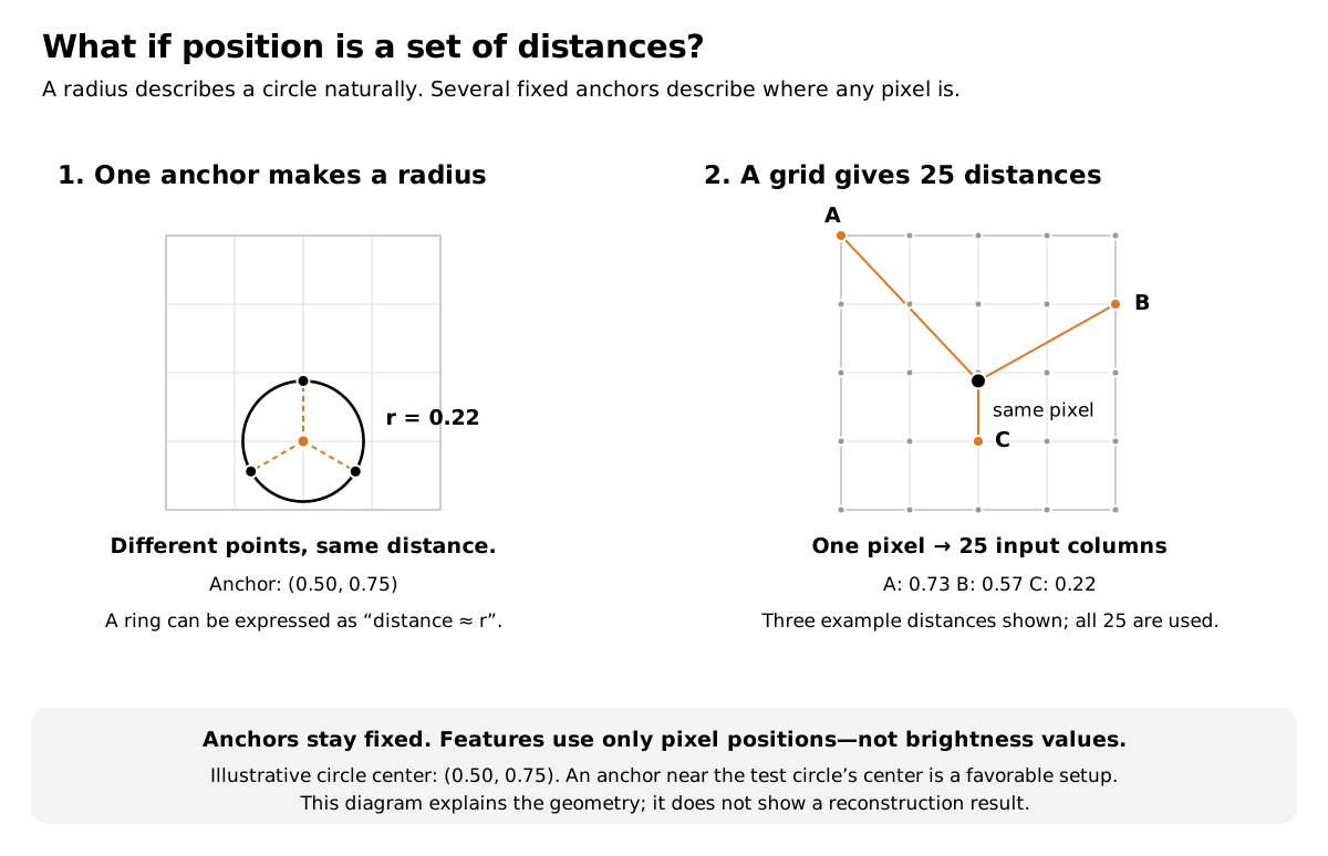
Each row now has 25 distance features. From a reference point near the center, the circle looks like a dark band at a particular distance.

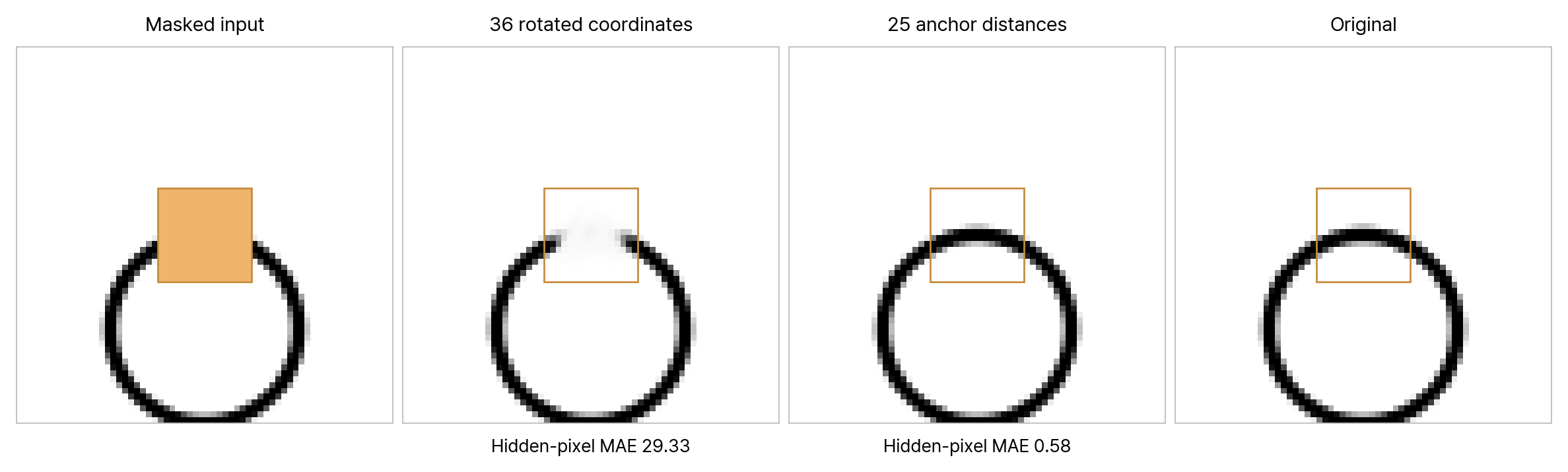
Causilo reconstructs the missing arc with distance features. MAE falls from 29.33 with rotated coordinates to 0.58 with distances.

The circle's center is close to one of the fixed grid points, so this example is well suited to these features. We would need to test other circle positions to see how consistently they help.

Can we use both feature sets in the same table?

Can one set of features handle both?

We combined them:

36 rotated-coordinate columns + 25 distance columns = 61 input columns.

Every pixel gets the same 61 features, for both the diagonal and the circle. Each image supplies its own visible brightness values as context.

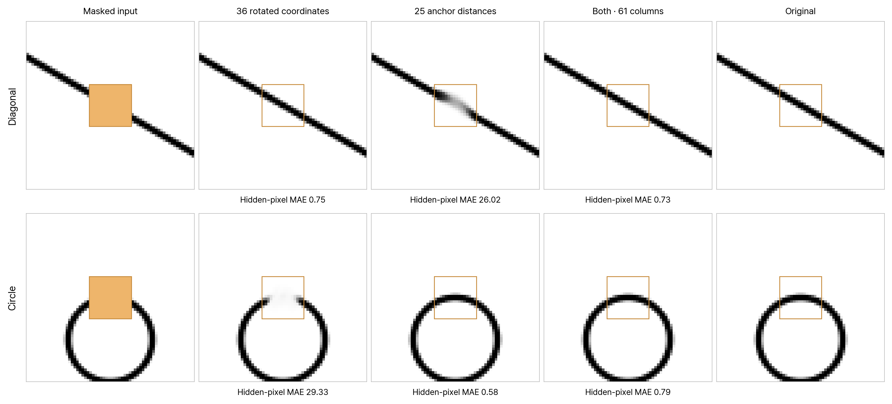
With both feature sets, Causilo reconstructs both shapes. MAE is 0.73 for the diagonal and 0.79 for the circle.

Distance alone gives a slightly lower error on this circle. Still, the combined features reconstruct both the diagonal and the arc with a single feature set.

Back to the photographs

We used the same representation for the face and tree at the start of this post. For color photographs, we predict red, green, and blue separately, then combine the predictions into an RGB image.

Each 256 × 256 photograph becomes a table:

• One row per pixel, with 61 positional features.
• A 16 × 16 hole leaves 65,280 visible rows as context.
• Causilo predicts 256 missing values per color channel.

All context rows come from the photograph being reconstructed. The hidden colors are used only to evaluate the predictions.

Here are four examples: the face and tree from the opening, a curved path through a lawn, and the edge of a car.

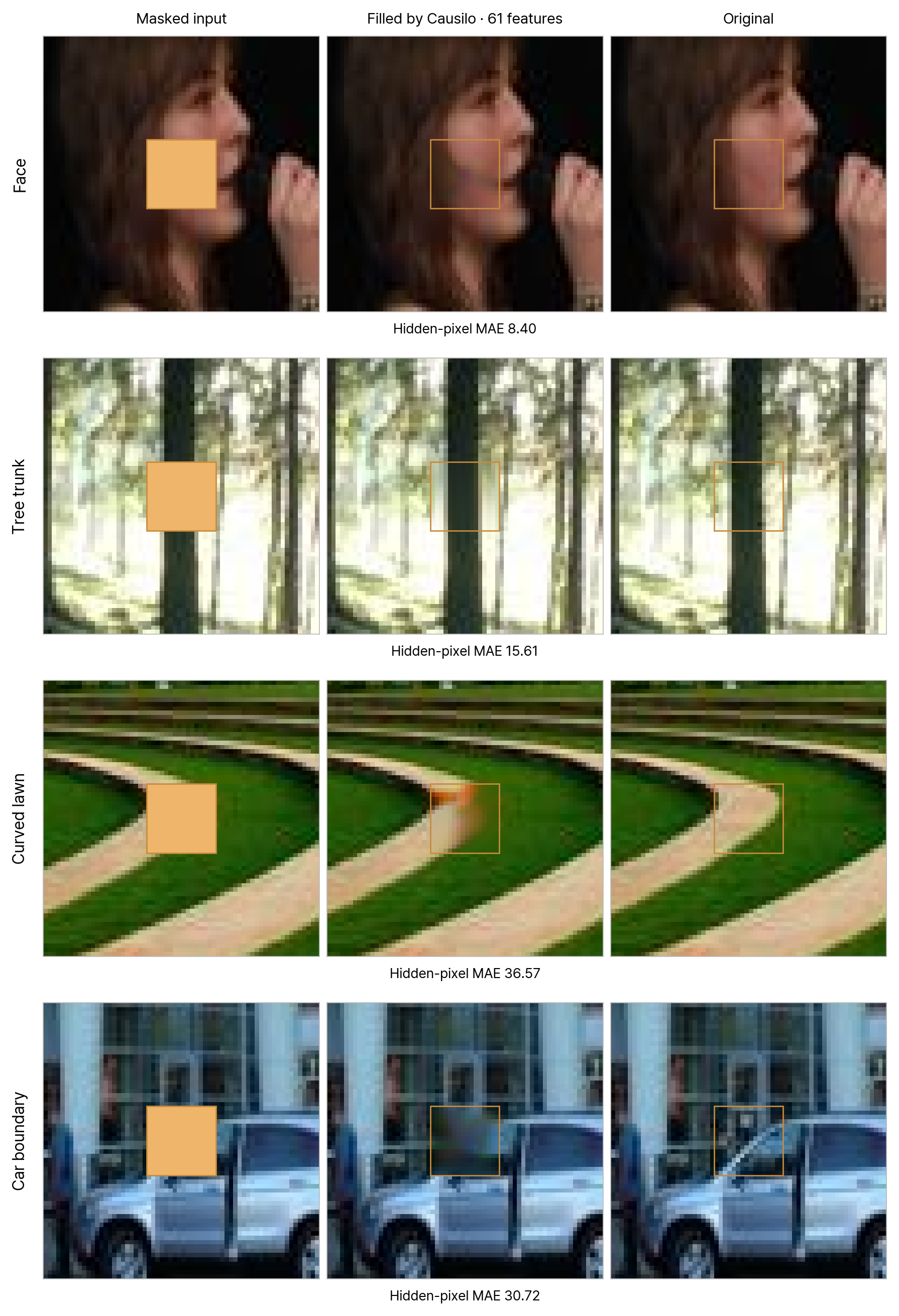
Each row shows a 64 × 64 close-up around the 16 × 16 missing region. Causilo predicts only the pixels inside the orange square.

Causilo fills the cheek with similar color and shading, and keeps the tree trunk recognizable. Both reconstructions lose fine texture.

On the lawn, the pale path continues into the gap, but the curve is distorted and its colors bleed into the grass. The clean circle was easier to reconstruct than this curved boundary in a photograph.

Several edges and surfaces meet inside the hole in the car image. Causilo fills it with colors similar to the surrounding pixels, but fails to reconstruct the sloping edge and finer details.

Causilo was pretrained entirely on synthetic tables. For this experiment, its only context was the visible pixels of each image. We supplied no additional photographs and did no fine-tuning for image completion.

With coordinates and distances as features, it reconnected a diagonal, completed a circular arc, and recovered recognizable structure in photographs. It used the visible parts of each image to make plausible predictions about what belonged in the gap.

These results surprised us. The reconstructions are imperfect, but they make us wonder: what else could a tabular foundation model do if we found the right way to represent the problem as a table?

---

Try the notebook

You can inspect the saved results in the Colab notebook. To reproduce them, save a copy to your Drive, select a T4 GPU, and run all cells. The notebook builds the features, runs Causilo, and evaluates the predictions.

The full photograph comparison

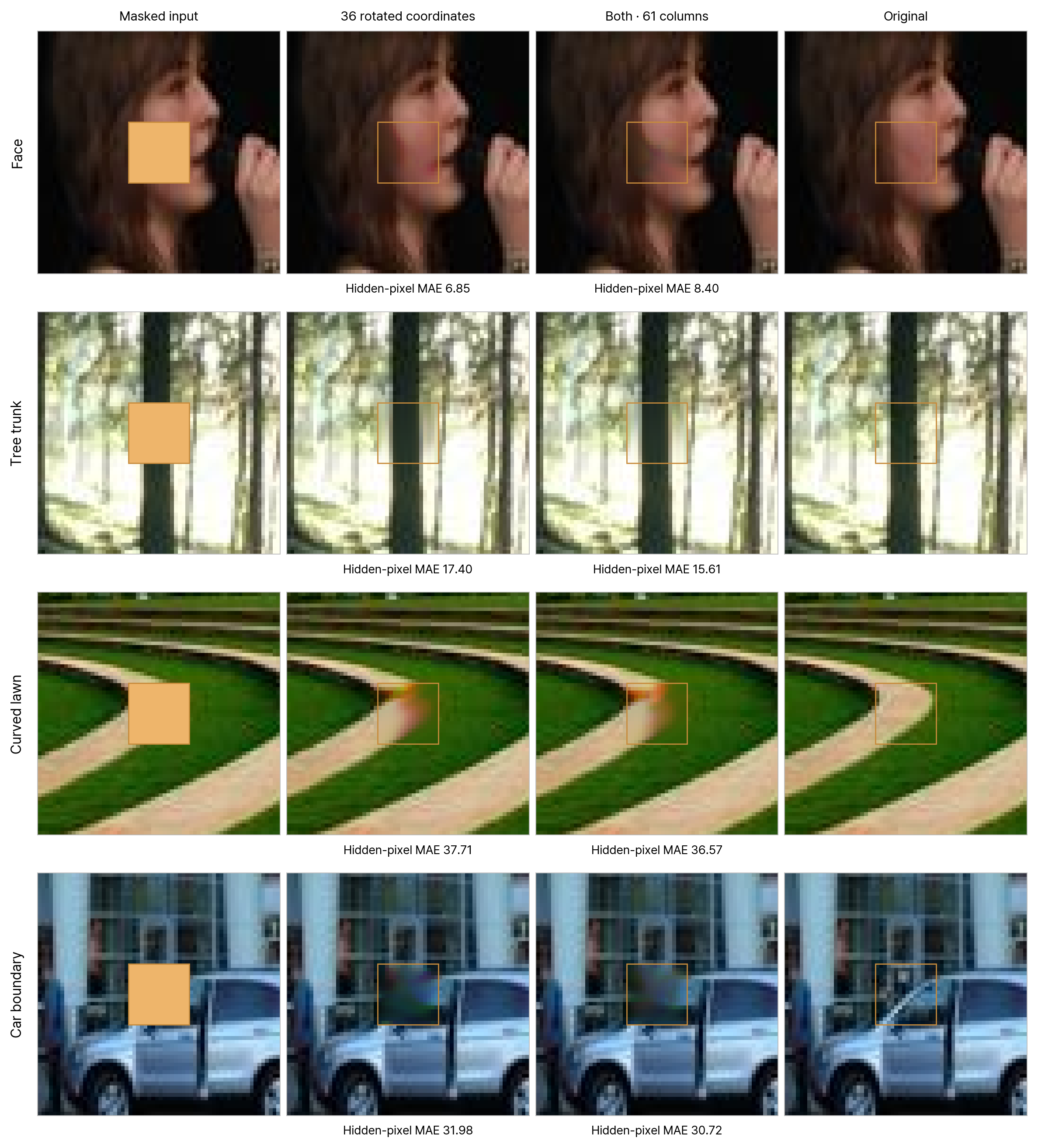
Missing region	Rotated coordinates: RGB MAE	Combined features: RGB MAE
Cheek	6.85	8.40
Tree trunk	17.40	15.61
Curved lawn	37.71	36.57
Car boundary	31.98	30.72

Errors are measured over the hidden pixels and all three color channels. Lower is better.

The opening images and the four-photo comparison both use the combined features. This table compares their errors with those from rotated coordinates alone; the close-ups show how the reconstructions differ.

Experiment notes

We used one fixed mask per image. These examples illustrate what Causilo can reconstruct under those settings; a broader study would be needed to assess performance across images or statistical significance. They also do not establish object recognition. We did not compare with a vision inpainting model.

All predictions use Causilo 1.0.2, one estimator, seed 20260928, and a Colab T4 GPU. We supply all visible pixels in a fixed shuffled order, clip predictions to 0–255, and evaluate errors only inside the hole.

The x,y, rotated-coordinate, and distance-only results come from earlier runs with matching inputs and settings. We ran the combined condition separately on the same images. A fresh notebook run recomputes every condition.

The four settings use 2, 36, 25, and 61 columns, so both the representation and feature count change. The diagonal is at an included angle of 30°, and the circle's center is close to a grid point. Other angles, circle positions, and mask locations need further testing.

The photographs are from the public Places365 validation archive. We selected the lawn image and mask before running its predictions. The notebook lists filenames, checksums, and mask positions for all four photographs, and verifies the downloaded JPEGs.